In ultrasonic ranging vehicle applications, such as: Ultrasonic Parking Assistance (UPA) and Blind Spot Detection (BSD), the ultrasonic waves emitted by the system are reflected back by surrounding objects. The system receives the reflected wave (echo) and then compares the echo amplitude of the object with a certain threshold to achieve the purpose of detecting the object. The closer an object is to the system, the stronger its echo. Therefore, the threshold varies with time and is a relatively common situation. This article will tell you that the threshold does not need to change and can remain fixed.
This article refers to the address: http://
Ultrasonic ranging
The Advanced Driver Assistance System (ADAS) used in cars is an ultrasonic ranging application. An ultrasonic sensor mounted on the front and rear bumpers and rearview mirrors of the vehicle emits ultrasonic waves and then receives ultrasonic waves reflected from surrounding objects. The propagation time of the ultrasonic wave (time of flight) is used to calculate the distance to the object to help the driver to park: find the parking spot, or detect objects in the driver's blind spot area. There are up to four sensors installed on the front and rear bumpers, and one sensor is attached to each rear view mirror.
In the ultrasonic advanced driver assistance system, a piezoelectric sensor is generally used to convert an electrical signal into an ultrasonic wave, and then convert the reflected ultrasonic wave into an electrical signal. The low receiver sensitivity of a piezoelectric ultrasonic sensor typically results in a very weak electrical signal when receiving reflected echoes.
Figure 1 shows a typical signal chain for processing echo voltages. The TI PGA450-Q1 is an integrated in-vehicle ultrasonic sensor signal conditioner for applications such as UPA systems.
Figure 1 ADAS for detecting objects using echo processing
The echo signal s(t) received by the ultrasonic receiver is corrupted by noise. The input-dependent noise η(t) shown in Figure 1 is the sum of the external ambient noise and all signal chain components, which is related to time (t). The corrupted signal u(t) is amplified by the amplifier using gain K and then digitized by an analog-to-digital converter (ADC). The digitized AM signal is transmitted by line through a bandpass filter (BPF). This filter is mainly used to improve the signal to noise ratio of the signal. The filtered signal y(t) is compared to a threshold L to detect the presence of an object. Behind the BPF there is typically an amplitude demodulator that converts the signal to baseband for comparison. However, for the convenience of this article, we have neglected this type of demodulator. Therefore, the key to detecting an object is the choice of threshold (L). So how do we choose L?
Echo amplitude
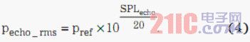
The ultrasonic waves generated by the transmitter are sinusoidal pulses at a range of carrier frequencies and are described in terms of sound pressure level (SPL). The SPL is calculated as follows:
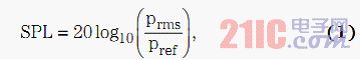
Among them, Prms is the RMS sound pressure, and pref is the reference sound pressure. The commonly used reference sound pressure is 20 μPa, or 0.0002 μbar.
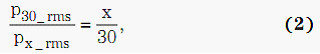
The ultrasonic SPL produced by the sensor on an object depends on the distance from the object to the sensor. In particular, please note that the sound pressure is inversely proportional to the distance:
Where p is the sonic pressure and d is the distance from the object to the sensor. The ultrasonic sensor specification describes the SPL at a distance of 30 cm. From this value, using this distance law, we can calculate the SPL of any distance x:
Where x is the distance between the sensor and the object and x > 30 cm. Therefore, the SPL for the x distance is:
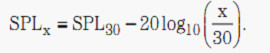
That is to say, when the ultrasonic wave propagates from the sensor to the object, the sound pressure is lost.
The sound waves are reflected back from the object and return to the sensor, and the sound pressure is further lost. In addition, since both air and objects absorb a part of the sound pressure, the SPL of the received echo can be approximated by Equation 3. The specific equation is shown at the end of the page. In the equation, α is the air absorption coefficient. Note that the SPL absorbed by the air is proportional to the distance the sound waves travel in the air. In other words, the SPL loss is proportional to x. We use a factor of 2 because the sound waves travel twice between the sensor and the object—from sensor to object, once from object to sensor. According to Equation 1, the sound pressure calculation method of the echo pulse received by the sensor is as follows:
The ultrasonic receiver converts the received sound waves into electrical signals. The conversion process is affected by receiver sensitivity (dB). Receiver sensitivity is 0 dB when 1 μPa sound pressure produces 10 V. Therefore, with Equations 5 and 6, the receiver sensitivity expressed in dB can be converted to V/μPa.
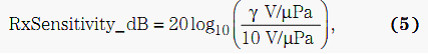
Where γ is the receiver sensitivity in units of V/μPa. Equation 5 can be rewritten as:
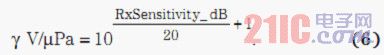
We can combine equations 4, 5, and 6 into equation 7 (see the end of this page) to calculate the voltage generated by the ultrasonic receiver. Equation 7 can be abbreviated as:
Among them, the gain (K) is a constant.
Equation 8 shows that as the distance x from the object increases, the echo voltage drops. In other words, the closer the object is, the larger the echo amplitude is, and the smaller the echo amplitude becomes when the object is far away.
Figure 2 shows that the received voltage is related to the distance from the object to the sensor, assuming the parameter values ​​are as follows:
SPL = 106 dB at 30cm distance
l Air absorption = 1.3 dB/m
l Object absorption = 0 dB
l Receiver sensitivity = –85 dB
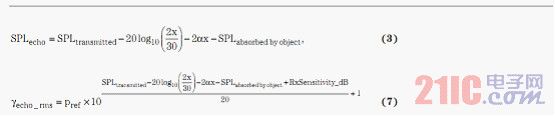
Figure 2 Receiver voltage as a function of object to sensor distance
Variable threshold scheme
The previous section shows that the amplitude of the echo received from the object decreases as the distance from the object to the sensor increases. In addition, as we know from Figure 1, the input signal of the echo processing path is u(t) = s(t) + η(t), where s(t) is the echo signal and η(t) is the input correlation noise. . In other words, the amplitude of the echo signal not only decreases with increasing distance, but also is destroyed by noise, and the echo processing system can only detect the presence of an object by processing the echo signal. A common method when selecting thresholds is the threshold scheme. When using this method, the threshold varies over time. In particular, when the ultrasonic wave is just emitted, the threshold is large, and thereafter, decreases as the elapsed time increases. The basic principle of this method is to use the predictable decay of the signal amplitude to determine the threshold size: the closer to the object, the larger the echo and the threshold, thus enabling object detection. The further away from the object, the smaller the echo and threshold.
Figure 3 depicts the concept of a variable threshold method. The figure shows an example of object echo demodulation at different distances. A test set for the TI PGA450-Q1 evaluation module is used to collect waveform data. This figure shows a possible threshold scheme.
Figure 3 Demodulated echo signal waveform for a possible threshold scheme
Although this variable threshold scheme approach is effective in principle, it has two drawbacks:
1. The variable threshold scheme requires memory inside the device to store the time and threshold relationship into the scheme table. If the threshold has 3 possible values ​​(as shown in Figure 3), the table will have 6 possible inputs. In addition, for the Advanced Driver Assistance System (ADAS) used in the vehicle, the user needs to enter a variety of possible sensor mounting positions, as the sensor can be mounted anywhere on the vehicle bumper or mirror. For example, if a sensor has 10 possible mounting locations, the device needs to store up to 60 location data. This increases the cost of the device because it requires more storage space.
2. After the sensor is installed on the car bumper and the mirror, the system manufacturer will “calibrate†the plan table. The calibration process is to determine the various thresholds and the time to switch the thresholds. This type of calibration is usually a time-consuming and costly task, especially if you need more than one input data in a table.
In summary, the main disadvantage of the variable threshold scheme is that it increases the total cost of the ultrasonic ranging system.
Fixed threshold
The variable threshold method uses a time-based threshold, which is not the same as this method. The fixed threshold method uses signal noise as a baseline. System noise is used to determine the threshold so that an object does not detect it if it does not exist.
In addition, as we know from Figure 1, the echo processing path input signal is u(t) = s(t) + η(t). The echo signal is a series of sine wave pulses at carrier frequency fc(t), which is calculated as follows:
Where S is the amplitude of the echo signal. Therefore, Equation 10 gives the RMS value of the amplified signal:
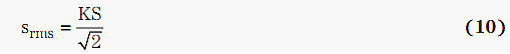
Note that this series of pulses appears only briefly, making the signal amplitude appear to be modulated for long periods of time.
The y (t) output of the bandpass filter (BPF) can be expressed as:
Among them, ƒ (BPF) is the digital filter function of BPF, and ƒ (ADC) is the quantization function of ADC. Assuming that the reference time of the echo signal is t0 = 0 (usually the time at which the transmitter emits ultrasonic waves), then y(t) < L, tend < t < tobject and y(tobject) ≥ L, and tend is greater than zero and is When the end of the initial burst of the pulse is transmitted, the presence of the object detected by the tobject can be declared. The question is, "Can we choose to use a fixed threshold and discard the variable threshold scheme?" To answer this question, we can use Equation 12 and assume that t is an instantaneous value to take care of the various noise components:
The variables are defined as follows:
K = amplifier gain
Ηext(t)=external noise
Ηamp(t)=Amplifier noise
ηADC(t) = ADC circuit noise
q(t) = ADC quantization
ηBPF(t) = BPF to calculate mathematical error
The individual noise components are not related to each other. In addition, we assume that each noise component has a zero mean and a non-zero variance Gauss.
Substituting Equations 9 and 12 into Equation 11, the BPF output becomes:
According to Equation 9, the RMS of the BPF noise is:
Where Q is the quality factor of the BPF, fs is the sampling frequency of the ADC, and all noise terms are RMS values. Knowing the RMS of the noise represented by Equation 14, and assuming a 6.6 crest factor, the selected threshold is:
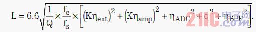
The above equation can be expressed as:
In other words, we can use Equation 15 to choose a fixed threshold. Figure 4 shows an example echo response using a fixed threshold.
Figure 4 Processing echo data using a fixed threshold
A significant advantage of using this method is that it only needs to store one input data. If a sensor has 10 possible mounting positions, only a total of 10 input data can be stored. Compared to the variable threshold approach described earlier, storage space requirements are reduced by a factor of 6. Note that Equation 15 also provides a mechanism to adjust the threshold if the amplifier gain (K) changes.
Equation 15 provides an analytical method for determining the threshold size. In general, noise analysis is needed to determine the threshold size. An alternative to noise analysis is to calibrate the sensors mounted on the vehicle using a threshold. The object can be placed at the farthest point of the sensor's specified ranging range, and then the ranging calibration is completed. The selected threshold should be large enough to exceed the noise value of the processed signal when there is no object and to ensure that the signal can pass through the threshold only when there is an object. Note that BPF attenuation should also be considered when using this method to select a threshold. Finally, in order to improve the robustness of the object detection system, the amplitude of the signal must be greater than a fixed threshold for a certain period of time.
This type of led power supply offers adjustable current for high mast lighting application with constant power(wide range selection),universal input voltage(90~!605Vac).Overall protection:Short circuit/Over temperature/Over Voltage.IP67, protect against more elements, suitable for dry/wet/damp location.0-10V&PWM dimmable,deliver maximun flrxibility with customized operating setting.Surge immunity: DM-5KV, CM-10KV.MOSO`s World wide distribution net gurrantee fast delivery&waranty service.
Approvals: in preparation if not already printed on product label.


High Mast Light LED Driver, LED High Power High Mast Driver,Outdoor High Mast Light LED Driver,Quality High Mast Light LED Driver
Moso Electronics , https://www.mosoleddriver.com